1 Approaching a design problem
Imagine your teacher says "build something cool" and walks away. No instructions! A bad student builds a random toy. A great student first asks lots of little questions — "Cool for who? How big? How fast?" — until they know exactly what to build, then builds it. A design interview is exactly that: the question is fuzzy on purpose, and your real job is to turn the fog into a clear plan before you build.
Before we touch a single trie or cache, we need to know how to attack an open-ended design question. This is a skill of its own — and it's very different from a coding (DSA) interview.
DSA interviews vs design interviews
| DSA interview | Design interview | |
|---|---|---|
| Problem statement | Concrete, well-defined | Extremely vague — e.g. just "Design Typeahead" (you might not even know what typeahead is) |
| Inputs / outputs | Example input-output pairs given | You have to figure them out |
| Direction | You know the kind of solution that works | Open-ended; discussion can go anywhere, depends on your and the interviewer's expertise |
| Constraints | Given (e.g. array of 10⁶ ints ⇒ can't use O(n²), max O(n log n)) | You must discover the constraints by asking |
| Time | Time constrained | Still time constrained — typically 45 mins |
Problem statement → work examples by hand → brute force → draw observations → optimize. A design interview borrows the spirit ("understand before you build") but the structure is different.
In a design interview your job is to (1) figure out what you're supposed to build — i.e. what the interviewer actually wants, (2) build that solution, and (3) deliberately take on sufficiently complex things so you can showcase your skills and impress the interviewer.
The 5-step design approach
A reliable script for the 45 minutes. Roughly the first half is about understanding, the second half about building.
Step 1 — Problem statement: reason by analogy
When the statement is vague, reason by analogy: find existing companies or systems that offer a similar product/feature. This gives you an overview of the umbrella of different scopes you could consider.
- Typeahead is a specific form of autocomplete — literally trying to type ahead of the user.
- Examples: typeahead in Google, typeahead in Amazon.
- Typeahead & Search are different products, but typeahead is always followed by some form of search.
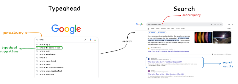
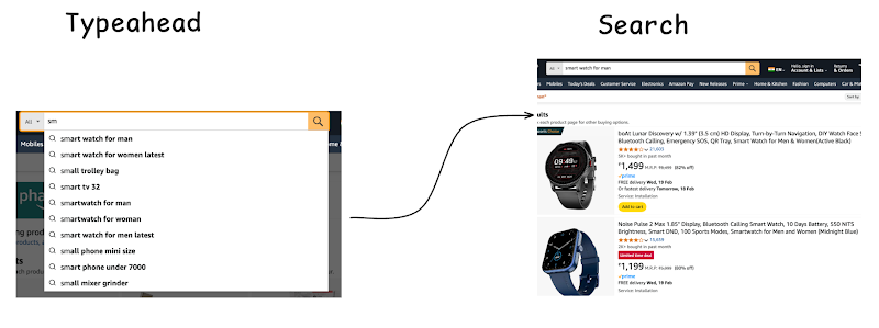
Autocomplete shows up in many settings, and most of them are not what we're designing:
- Smartphone keyboards: word completion / contacts.
- Text / code editors: intellisense (complete next token), GitHub Copilot (whole functions).
- Grammarly: sentence completion while writing prose.
- Gmail / Outlook: sentence completion for mail; to/cc/bcc email completion from contacts.
The key difference: autocomplete is typically local to your machine and standalone — suggestions are specific to you. Typeahead is always associated with search, and its suggestions are the most popular queries searched globally in the past that match the given prefix.
Functional requirements & the MVP mindset
Functional requirements (FR) start from a Minimal Viable Product (MVP):
- Minimal: the minimal set of features to achieve viability.
- Viable: should demonstrate the core features & usability.
- Product: solve a genuine problem.
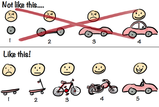
Always keep "minimal" in mind — MVP features is not a feature-suggestion competition. Features fall into three buckets:
| Bucket | Meaning | Verdict |
|---|---|---|
| MVP (v0) | Core features — perfect for discussion | ✅ build & discuss |
| Future scope (v1+) | Good to have, not absolutely necessary | 🟡 mention, don't build |
| Bad (v-never) | Gets you rejected in an interview | ❌ avoid |
Don't propose anything that doesn't affect our backend infra / system design:
- Frontend / purely cosmetic features that don't affect backend design.
- Common dependencies that aren't the core of the system. E.g. designing Uber needs authentication and payments — but auth isn't what you're asked to design, it's just a dependency. Assume auth & payments already exist.
Also: any suggested feature should come as a complete sentence from the user's perspective.
For every feature you discuss, think about its API — is it user-facing or internal? That question surfaces features you'd otherwise miss. For typeahead:
typeahead(partial_query) => suggestions_list   # user-facing
log_search(search_query)  => void              # internal
2 Requirements & scale
Imagine a super-helpful librarian who has heard every question anyone has ever asked. The moment you open your mouth and say "how do I tie…", she instantly blurts out the most common ways people finish that sentence — "…tie a tie?", "…tie my shoes?" She's so fast it feels like she's reading your mind, and she only suggests things lots of people actually ask. That librarian is autocomplete.
Before designing anything, a good engineer writes down what the system must do. We split this into two buckets. Functional requirements are the features — what the user can see and do. Non-functional requirements are the qualities — how fast, how reliable, how big. Autocomplete is a fascinating case study because its features are tiny but its quality bar is brutal.
There's exactly one actor to keep in mind here: the end user — the person doing the Google search.
Functional requirements (what it does)
Stated as complete user-perspective sentences: "As the user is typing in the search box, we should auto-complete their search query — we should show typeahead suggestions."
- Prefix suggestions. Given a prefix /
partial_query(the letters typed so far, like"how to ti"), return a list of complete queries that start with those letters — the user-facing APItypeahead(partial_query) => suggestions_list. - Suggestions are popular past searches. The list comes from searches other
people made before, captured via the internal API
log_search(search_query) => void. - Ranking by popularity (top 5, relevant). We show only the
top 5 relevant suggestions. Relevant = the suggestion is a
prefix match with the
partial_query. Top 5 = we track how many times eachsearch_queryhas been searched globally, and among prefix matches we show those with the highest count. - Update on every keystroke. With every letter the user types, the suggestions change — we send a new API request with every letter typed.
- Clicking a suggestion triggers a search (frontend).
Scope boundaries we picked
- Start at ≥ 3 letters. We only start showing suggestions after the user has typed at least 3 letters — fewer than that gives irrelevant results.
- Cap at 50 letters. If a query is longer than ~50 letters, the user has most likely fallen asleep on the keyboard.
Nice-to-haves that we deliberately defer: personalization (by geolocation, the user's own browsing/search history, even age — "why is s…" → "why is sky blue" for a 5-year-old vs "why is scotch smooth" for a 30-year-old); recency / trending news factor; showing trending or recent searches even before 3 characters; spell-correction and grammar-correction of the partial query; Tab to copy a suggestion into the box; highlighting the already-typed part; and "provide suggestions as per the law of the land" (whatever that means).
The qualities (latency, consistency, availability) and the numbers (QPS, storage, sharding) are big enough to deserve their own sections — see §4 Non-functional requirements and §5 Scale estimation below. First, though, we sketch the API and where the data comes from.
3 API & data flow
Two friends pass notes. You hand the librarian a slip with the start of your question and she hands back a list — that's one note ("give me suggestions"). Separately, every time anyone asks a full question, a helper quietly tells the librarian "someone asked this" so she can keep her tallies — that's a second, behind-the-scenes note. Same idea, two different notes.
For each feature, decide its API — its input & output (the interface) — and its protocol — how the communication happens (REST / RPC / …). Those are two different things.
typeahead(partial_query) => suggestions_list      # user-facing
log_search(search_query)  => void                 # internal

GET /typeahead?partialQuery={...}                 # the HTTP shape
Design questions worth raising aloud in the interview: why REST (not SOAP / RPC / …)?
and why GET (not POST)? — naming conventions and idempotent reads point to a cacheable
GET.
Where do the suggestions come from?
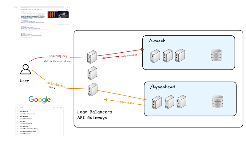
Users are constantly searching on Google. The data flow that feeds typeahead:
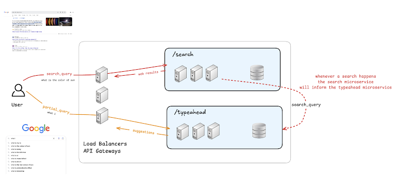
Crucially, step 3 is asynchronous — the user's search isn't slowed down by logging.
The /typeahead microservice is fed by the /search
microservice rather than living on the search path.
typeahead(partial_query) exposed as a cacheable
GET /typeahead, and internal log_search(...).
API ≠ protocol. Suggestions are populated when /search
asynchronously informs /typeahead of each search.
4 Non-functional requirements
Two questions about the librarian, besides what she does: Is it okay if she's sometimes a tiny bit out of date with her tallies? (Yes — nobody knows or cares about the exact counts.) And how fast must she be? (Faster than you can type the next letter!) Those two answers — "stale is fine" and "be lightning fast" — decide almost everything about how we build her.
Non-functional requirements (NFR) are our design goals. The right tool to reason about them is PACELC: in a Partition, choose Availability or Consistency; Else (normal operation), choose Latency or Consistency. Do NOT jump to an answer — reason it out.
Consistency vs Availability
Q: What is the data? Past search queries and their corresponding counts.
| Search Query | Count |
|---|---|
| why is the sky blue? | 49,999 |
| why is water wet? | 50,000 |
| what is the color of the ocean | 5,000 |
Q: What does eventual consistency mean here? When is the data changing? Every time
someone searches, some entry's count changes, and the top-5 for some partial_query
may change. It's possible for a new count to reflect in the top-5 with a delay — for some time the true
count of Query1 may exceed Query2, yet we still show Query2 first.
The user doesn't know (or care about) the true search counts. We don't need a strict order in the suggestions, and it's fine for a few good suggestions to be missing as long as the ones shown are also good enough. So we lean toward availability over strict consistency.
Q: What does data loss mean here? If someone searched but, for whatever reason, we failed to increment that query's count (it didn't get logged), the counts will be off by a small amount:
| Search Query | True Count | DB Count |
|---|---|---|
| why is suryakumar dropped? | 49,999 | 49,999 |
| why is water wet? | 50,000 | 49,998 (lost a few) |
| what is the color of the ocean | 5,000 | 5,000 |
Same reasons as stale reads: being off by a small amount in the counts doesn't hurt the user experience.
Consistency vs Latency
We're literally competing with the user's typing speed. Target: each typeahead query takes < 10 ms. Note this excludes the network round trip, which depends on the user's distance from the servers — we don't control that, and the only fix is geolocated servers.
Other NFRs (briefly)
- Security: do NOT roll your own unless you're a security expert — "99% of security issues happen because non-experts try to do security."
- Observability, rate limits, idempotency, and delivery guarantees are worth a mention.
People read suggestions far more than the popular-query set changes. So this is an overwhelmingly read-heavy system — which (combined with "stale is fine") is why we precompute answers and cache aggressively rather than calculate live.
5 Scale estimation
Before building a bridge you guess how many cars will cross it — not the exact number, just "thousands? millions?" If millions, you build a very different bridge. We do the same: rough math to learn whether one librarian can cope, or whether we need a whole building full of them.
The scale dictates our design choices. We want to know: the amount of data (is sharding needed?), and the amount of load (requests/second per API, peak vs average, read- vs write-heavy). Those guide the choice of database, cache and sharding.
These are back-of-the-envelope estimates. Being off by a factor of 2 or 3 is fine (true 100 → you say 50 or 200, okay; you say 10, not okay — off by 10×). But every estimate must be justified — don't pull numbers from thin air, and state every assumption as an assumption.
Step 1 — Daily Active Users
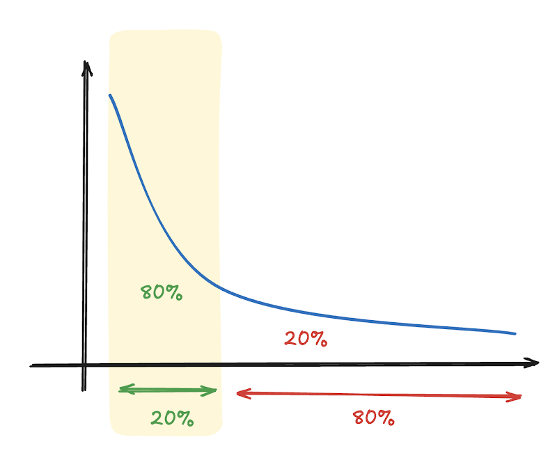
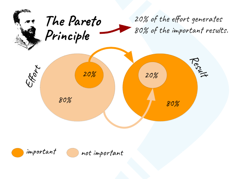
Handy reference numbers: world population ~8 billion; internet users ~5 billion; India ~1.4 billion; USA ~350 million. And the Pareto principle (80/20): only ~20% of users are active. (For social media it extends to 80-20-1: 80% passively browse, 20% interact, 1% create.)
# Assumption: Google has 5 billion users.
DAU            = 20% of 5 billion        = 1 billion users

# Assumption: 20 searches / active user / day
searches/day   = 20 * 1 billion          = 20 billion searches/day

# 1 day = 86,400 s ~= 10^5 s
searches/sec   = 20*10^9 / 10^5          = 200,000 searches/sec
# note: these go to the SEARCH api, not typeahead

# Assumption: ~10 typeahead calls per search
# (avg query ~10 letters, start at letter 3 => 10-3=7 ~ 10)
typeahead/sec  = 200,000 * 10            = 2,000,000 typeaheads/sec

log_search/sec = 1 per search            = 200,000 req/sec

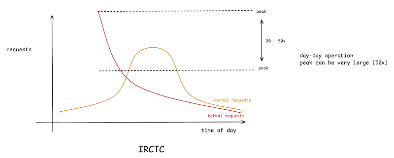
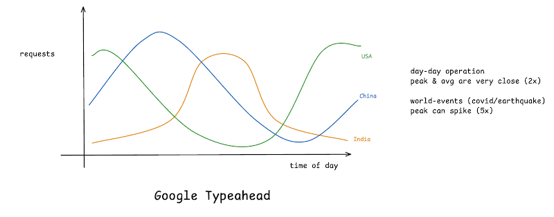
# Peak load ~= 5x average
peak typeahead = 5 * 2,000,000           = 10,000,000 typeaheads/sec
Why ~10 typeaheads per search: typing "why is the sky blue" fires
typeahead("why"), typeahead("why i"),
typeahead("why is"), … one per keystroke after the third letter.
Step 2 — Amount of data
The data is past search queries & their counts (avg query size 10 letters, assumed earlier). How many entries? Not one per search — repeated searches just update a count; only new (never-seen-before) unique queries add rows.
# Assumption: ~10% of searches are brand-new queries
new entries/day = 10% of 20 billion      = 2 billion entries/day

# ~10 bytes per entry
data/day        = 10 bytes * 2 billion   = 20 GB / day

# over 20 years (365 ~= 400 days)
total           = 20 GB/day * 20*400 days
                = 16 * 10^4 GB           = 160 TB
Can 160 TB fit on a single server? Probably yes with modern storage. But can a single server handle 10 million requests/second? Absolutely not. So sharding is required — driven by load, not storage.
Step 3 — Read-heavy or write-heavy?
| API | Type | Rate |
|---|---|---|
typeahead | read | 2,000,000 req/sec |
log_search | write | 200,000 req/sec |
Reads are 10× writes, so we call this read-heavy — even though the writes are themselves significant.
When a system is read-heavy and the writes are also significant: absorb the reads in a cache, and optimize the database for writes. No database is optimized for both reads and writes — that's impossible.
log_search/sec.
Storage ~160 TB over 20 years. The 10M QPS (not the storage) forces
sharding. Reads are 10× writes ⇒ read-heavy ⇒ cache the reads, optimize
the DB for writes.
6 The Trie data structure
Think of a giant family tree, but for words. At the very top is "nothing." Below it are 26 branches, one for each first letter. Follow the "c" branch, then "a," then "t," and you've spelled "cat." Every word that starts with "ca" — cat, car, cake — lives down the same "c → a" hallway. So if you only know the start of a word, you just walk down that hallway and collect everything hanging below. That word-tree is called a trie.
A trie (pronounced "try," from retrieval — also called a prefix tree) is a tree where each edge represents one character and each path from the root spells out a prefix. It's the natural fit for autocomplete because finding "all words starting with P-R-E" is just "walk to the node at the end of PRE, then look below."
How terms are stored
Every node in the trie holds a map from a character to a child node. To store
the word "cat," we walk/create children c → a → t and mark the final node as the
end of a real word. To store "car" too, it shares the c → a path and only
branches at the third letter. Shared prefixes = saved space.
Insertion and lookup
Insertion: walk the word letter by letter, creating any missing child nodes, and mark the last node as a word-end. Lookup of a prefix: walk the prefix letter by letter from the root; if you ever can't find the next child, there are no matches. If you reach the end of the prefix, the node you land on is the root of a subtree containing every word with that prefix.
# Python — trie with per-word frequency + top-k prefix query
import heapq

class TrieNode:
    def __init__(self):
        self.children = {}        # char -> TrieNode
        self.is_word  = False
        self.word     = None      # full word, set at the end node
        self.freq     = 0         # search frequency of this word

class Trie:
    def __init__(self):
        self.root = TrieNode()

    def insert(self, word, freq=1):
        node = self.root
        for ch in word:                 # walk/create the path
            if ch not in node.children:
                node.children[ch] = TrieNode()
            node = node.children[ch]
        node.is_word = True
        node.word    = word
        node.freq   += freq               # aggregate repeated inserts

    def _find(self, prefix):              # walk to the prefix node
        node = self.root
        for ch in prefix:
            if ch not in node.children:
                return None          # no words with this prefix
            node = node.children[ch]
        return node

    def suggest(self, prefix, k=5):
        node = self._find(prefix)
        if node is None:
            return []
        matches = []
        stack = [node]
        while stack:                       # gather every word under the prefix
            cur = stack.pop()
            if cur.is_word:
                matches.append((cur.freq, cur.word))
            stack.extend(cur.children.values())
        # top-k by frequency (descending)
        best = heapq.nlargest(k, matches)
        return [(w, f) for f, w in best]

# --- demo ---
t = Trie()
for w, f in [("cat", 8), ("car", 5), ("card", 3),
              ("care", 9), ("dog", 4)]:
    t.insert(w, f)
print(t.suggest("ca", 3))    # [('care', 9), ('cat', 8), ('car', 5)]
// C++ — trie with per-word frequency + top-k prefix query
#include <bits/stdc++.h>
using namespace std;

struct TrieNode {
    unordered_map<char, TrieNode*> children;  // char -> child
    bool   isWord = false;
    string word;                              // set at the end node
    long   freq  = 0;                          // search frequency
};

struct Trie {
    TrieNode* root = new TrieNode();

    void insert(const string& word, long freq = 1) {
        TrieNode* node = root;
        for (char ch : word) {              // walk/create the path
            if (!node->children.count(ch))
                node->children[ch] = new TrieNode();
            node = node->children[ch];
        }
        node->isWord = true;
        node->word   = word;
        node->freq  += freq;                  // aggregate repeated inserts
    }

    TrieNode* find(const string& prefix) {  // walk to the prefix node
        TrieNode* node = root;
        for (char ch : prefix) {
            auto it = node->children.find(ch);
            if (it == node->children.end()) return nullptr;
            node = it->second;
        }
        return node;
    }

    vector<pair<string, long>> suggest(const string& prefix, int k = 5) {
        vector<pair<string, long>> matches;
        TrieNode* start = find(prefix);
        if (!start) return matches;
        vector<TrieNode*> stack{start};
        while (!stack.empty()) {              // gather every word under the prefix
            TrieNode* cur = stack.back(); stack.pop_back();
            if (cur->isWord) matches.push_back({cur->word, cur->freq});
            for (auto& [c, child] : cur->children) stack.push_back(child);
        }
        // top-k by frequency (descending)
        sort(matches.begin(), matches.end(),
             [](const auto& a, const auto& b){ return a.second > b.second; });
        if ((int)matches.size() > k) matches.resize(k);
        return matches;
    }
};

int main() {
    Trie t;
    t.insert("cat", 8); t.insert("car", 5); t.insert("card", 3);
    t.insert("care", 9); t.insert("dog", 4);
    for (auto& [w, f] : t.suggest("ca", 3))
        cout << w << " " << f << "\n";  // care 9 / cat 8 / car 5
}
// Java — trie with per-word frequency + top-k prefix query
import java.util.*;

class TrieNode {
    Map<Character, TrieNode> children = new HashMap<>();  // char -> child
    boolean isWord = false;
    String  word;                                       // set at the end node
    long    freq = 0;                                    // search frequency
}

class Trie {
    private final TrieNode root = new TrieNode();

    void insert(String word, long freq) {
        TrieNode node = root;
        for (char ch : word.toCharArray())            // walk/create the path
            node = node.children.computeIfAbsent(ch, c -> new TrieNode());
        node.isWord = true;
        node.word   = word;
        node.freq  += freq;                            // aggregate repeated inserts
    }

    private TrieNode find(String prefix) {            // walk to the prefix node
        TrieNode node = root;
        for (char ch : prefix.toCharArray()) {
            node = node.children.get(ch);
            if (node == null) return null;       // no words with this prefix
        }
        return node;
    }

    List<Map.Entry<String, Long>> suggest(String prefix, int k) {
        List<Map.Entry<String, Long>> matches = new ArrayList<>();
        TrieNode start = find(prefix);
        if (start == null) return matches;
        Deque<TrieNode> stack = new ArrayDeque<>();
        stack.push(start);
        while (!stack.isEmpty()) {                      // gather every word under the prefix
            TrieNode cur = stack.pop();
            if (cur.isWord)
                matches.add(Map.entry(cur.word, cur.freq));
            for (TrieNode child : cur.children.values()) stack.push(child);
        }
        // top-k by frequency (descending)
        matches.sort((a, b) -> Long.compare(b.getValue(), a.getValue()));
        return matches.subList(0, Math.min(k, matches.size()));
    }
}

public class Demo {
    public static void main(String[] args) {
        Trie t = new Trie();
        t.insert("cat", 8); t.insert("car", 5); t.insert("card", 3);
        t.insert("care", 9); t.insert("dog", 4);
        System.out.println(t.suggest("ca", 3));
        // [care=9, cat=8, car=5]
    }
}
The clever bit: store top-k at each node
Here's the trick that makes autocomplete fast. The naive way is: walk to the prefix node, then explore the whole subtree below it to gather all matching words and sort them by popularity. For a popular prefix like "a," that subtree is enormous — far too slow per keystroke.
Instead, we precompute and cache the top-k suggestions directly on every node (the
top_k list above). When we build the trie offline, each node already carries a
ready-made answer: the k most popular complete queries that pass through it. Now a lookup is just "walk to
the node, read its list." No subtree exploration at request time.
The node for prefix "how to ti" might store, already sorted by popularity:
node["how to ti"].top_k = [
    ("how to tie a tie",   980000),
    ("how to tie shoes",   540000),
    ("how to title a paper",120000),
    ("how to time a roast", 30000),
]
A request for that prefix returns this list instantly — the ranking work was done ahead of time.
Complexity (the Big-O)
| Operation | Cost | Why |
|---|---|---|
| Insert a word of length L | O(L) | One step per character. |
| Look up a prefix of length P | O(P) | Walk P characters from the root. |
| Get top-k (with precomputed lists) | O(P + k) | Walk to the node, copy its k items. |
The beautiful part: lookup cost depends only on how long the prefix is, not on how many millions of queries are stored. Typing 9 characters costs 9 steps whether the trie holds a thousand words or a billion. That's why a trie hits our latency target.
Storing a top-k list on every node uses a lot of memory (we're trading space for speed — a recurring theme in HLD). And because the lists are precomputed, the trie is essentially read-only at serving time: you don't edit it live, you rebuild it offline (next section).
7 Ranking & data collection
Imagine the librarian keeps a tally chart. Every time someone asks a question, she adds a tick mark next to it. When you start a question, she suggests the ones with the most ticks first — because lots of people asking it probably means it's what you want too. And she slowly fades old tick marks so last year's hot question doesn't beat today's. That tally chart is how she ranks.
In Section 2 we waved our hands and said each node "knows" its top-k. Now we earn that. Where do the popularity numbers come from, and how do we keep them current?
Ranking by frequency and recency
The simplest signal is frequency: how many times has each full query been searched? More searches → higher rank. But pure frequency makes the list stale — an all-time favorite would cling to the top forever. So we add recency: recent searches should count for more than ancient ones.
A common technique is a time-decayed score: every day, multiply all existing counts by a factor like 0.95, then add today's fresh counts. Old popularity gently fades; trending queries rise. The final rank for a query is just this decayed score.
Query "world cup schedule" with a daily decay of 0.95:
# score_today = score_yesterday * decay + searches_today
Day 1:   0      * 0.95 + 100  = 100
Day 2:   100    * 0.95 +  50  = 145
Day 3:   145    * 0.95 +   0  = 138   # no searches: fades
Day 4:   138    * 0.95 + 900  = 1031  # goes viral: jumps up
Notice a once-popular query naturally decays when interest dies, and a sudden spike quickly lifts it. This keeps suggestions feeling alive without us hand-curating anything.
How query logs feed popularity
Every search a user runs is recorded in a query log — append-only lines of "this query was searched at this time." At our scale that's billions of lines a day, far too much to count live on the serving path. Instead the logs stream into a message queue (think of a conveyor belt like Kafka) and pile up in cheap storage for batch processing.
Updating a live ranking on every single search would put writes on the hot read path and wreck our latency — exactly the read-heavy lesson from Section 1. Decoupling "collect now, compute later" keeps the fast serving path read-only and lets the heavy counting happen safely off to the side.
The offline aggregation pipeline
This is the offline pipeline — a scheduled job (say, hourly) that turns raw logs into a fresh trie. "Offline" means it runs separately from live traffic; users never wait on it.
Step 3 is typically a MapReduce-style job: "map" each log line to
(query, 1), then "reduce" by summing per query and applying decay. Step 4 builds a
fresh trie and, while building, computes each node's top-k by merging the top-k of its children (a child's
best suggestions are candidates for the parent). Step 5 atomically swaps the new trie in for the old one.
# A node's best suggestions come from merging its
# children's best suggestions, plus its own word if any.
def compute_top_k(node, k=5):
    candidates = []
    if node.is_word:
        candidates.append((node.word, node.score))
    for child in node.children.values():
        compute_top_k(child, k)          # bottom-up
        candidates.extend(child.top_k)
    # keep only the k highest-scoring
    node.top_k = sorted(candidates, key=lambda x: -x[1])[:k]
Because each node only keeps its k best, the merge stays cheap even near the root.
Ranking is a blend of frequency and recency (time-decayed scores), and it's computed offline from query logs, never on the live request. The serving trie is just a frozen snapshot of "what's popular right now," rebuilt and swapped in periodically — the same prefill-then-serve spirit you'll see all over HLD.
8 Serving at scale
One librarian can't answer a whole stadium at once. So we hire many identical librarians (copies), put a greeter at the door to send each person to a free one (load balancing), and split the giant book collection alphabetically across rooms so no single room is overwhelmed (sharding). We also keep a cheat-sheet of the most-asked questions right at the front desk (caching), and we politely ask you to finish a few letters before we run off to fetch an answer (debouncing). Together they keep everyone served in a blink.
We now have a fast trie (Section 2) kept fresh by an offline pipeline (Section 3). The last job is delivering it to ~400k QPS with sub-100 ms latency. We reuse the big HLD building blocks from earlier sessions.
Caching hot prefixes
A tiny fraction of prefixes accounts for a huge fraction of traffic — single letters and common starts like "f," "you," "how to." We put a cache (a fast in-memory key→value store like Redis, recall the caching session) in front of the trie, keyed by prefix. The first lookup of "how to" computes the answer; the next million read it straight from cache.
Suggestions for "how to" are identical for everyone and change only when we rebuild the trie. That makes them perfect cache entries: same input → same output, rarely changing. A cache hit avoids even the cheap trie walk and shaves precious milliseconds. We set a short TTL (time-to-live) so the cache refreshes after each trie rebuild.
Sharding the trie
Our 10 GB trie fits in one machine's RAM, but one machine can't handle 400k QPS alone. So we shard (split the data across machines, recall the sharding session). The natural key is the prefix's first letter(s): shard A handles prefixes starting "a," shard B handles "b," and so on. A request for "how to ti" is routed to the "h" shard.
Naive first-letter sharding is uneven — far more queries start with "s" than "z," so the "s" shard melts while "z" sits idle. Fixes: shard on the first two or three letters for finer slices, or use consistent hashing to spread load evenly. And because the trie is read-only at serving time, we can freely keep multiple replicas of each shard to share the read load — read-heavy systems love replication.
CDN and edge
The fastest request is the one that never reaches your servers. A CDN (Content Delivery Network — a fleet of caches physically close to users) and edge nodes can cache the suggestions for the most common prefixes right next to the user, in their region. Latency is dominated by physical distance, so answering "how to" from a city 50 km away instead of a data center 5,000 km away is a giant win for our latency budget.
Debouncing on the client
Half of our scaling problem can be solved in the browser. Debouncing means: don't fire a request on every keystroke — wait until the user pauses typing (say 150–300 ms) and only then send the latest prefix. A fast typer entering "how to tie" generates one request instead of ten.
let timer;
input.addEventListener("input", () => {
  clearTimeout(timer);                  // cancel the pending request
  timer = setTimeout(() => {            // wait for a pause
    fetchSuggestions(input.value);      // only the latest prefix is sent
  }, 200);                            // 200 ms of quiet
});
This alone can cut autocomplete QPS several-fold — the cheapest scaling lever we have, and it lives entirely on the client.
The end-to-end request flow
Putting every block together, here's the journey of one keystroke from your keyboard to a dropdown:
Each layer is an opportunity to answer early: the request stops at the first layer that already knows the answer. Most requests never reach the trie at all — they're caught at the edge or in the cache. That layered, "answer as early as possible" shape is the heart of serving any read-heavy system at scale.
From Section 1, autocomplete is a nice-to-have. If the suggestion service is overloaded or down, the page should simply show no dropdown and let the user search normally — never block the search box. Designing the failure to be invisible is just as important as designing the success.
★ Putting it all together
You just designed a real, production-grade system end to end. Here's the one-paragraph story that connects all four topics:
Autocomplete must return the top-k most popular queries for a typed prefix in under ~100 ms at hundreds of thousands of QPS — a read-heavy problem whose data is small enough to live in RAM. We store the queries in a trie and precompute each node's top-k so a lookup is a quick O(P+k) walk-and-read. Those popularity numbers come from query logs, turned into time-decayed rankings by an offline pipeline that periodically rebuilds and publishes the trie. Finally we serve it at scale by stacking debouncing, CDN/edge, load balancing, caching of hot prefixes, and a sharded, replicated trie — each layer answering as early as it can, and failing gracefully when it can't.
Quick self-check
What are the 5 steps of the design approach, and how is the 45 min split?
(1) Problem statement, (2) Functional requirements, (3) Non-functional requirements, (4) Scale estimation, (5) API + System design. Roughly the first 20–25 min on steps 1–4 (understanding), the remaining 20–25 min on step 5 (building).
How is typeahead different from general autocomplete?
Autocomplete (keyboards, IDEs, Grammarly, Gmail) is usually local/standalone and personal to you. Typeahead is always tied to search, and its suggestions are the most popular queries searched globally in the past that prefix-match what you typed.
Can the typeahead system tolerate stale reads and small data loss? Why?
Yes to both. Users don't know or care about the true search counts, and we don't need a strict ordering — a few good suggestions missing is fine as long as the shown ones are good enough. So we favor availability/eventual consistency.
Walk the load estimate: from DAU to peak typeahead QPS.
5B users × 20% = 1B DAU; × 20 searches/day = 20B searches/day ÷ 10⁵ s ≈ 200k searches/sec; × ~10 typeaheads/search = 2M typeaheads/sec; × 5 peak factor = ~10M typeaheads/sec at peak. (log_search ≈ 200k/sec.)
Why is autocomplete described as a "read-heavy" system, and why does that matter?
Users read suggestions billions of times a day, but the popular-query set changes slowly, so there are far more reads than writes. That justifies precomputing answers, caching aggressively, and replicating the read-only trie.
What is the time complexity of a prefix lookup in a trie, and what does it depend on?
O(P) to walk the prefix (plus O(k) to copy the precomputed suggestions). It depends only on the prefix length P, not on how many millions of queries are stored — which is why it's fast at any scale.
Why precompute top-k on each node instead of searching the subtree at request time?
Exploring the whole subtree below a popular prefix (like "a") is far too slow per keystroke. Precomputing the top-k offline turns the request into a cheap walk-and-read, trading extra memory for speed.
How do we keep suggestions fresh without slowing down live requests?
Capture searches in query logs, then run an offline pipeline that aggregates them with a time-decayed score, rebuilds the trie, and swaps it in periodically. All the counting happens off the hot read path.
Naive first-letter sharding overloads some shards. Name two fixes.
(1) Shard on the first two or three letters for finer, more even slices; (2) use consistent hashing to distribute load evenly. Also replicate each read-only shard to share the read load.
What is debouncing and why is it the cheapest scaling lever?
Debouncing waits for a short typing pause before sending only the latest prefix, instead of firing on every keystroke. It can cut QPS several-fold and lives entirely on the client — no server cost.
📚 References & Further Reading
Class material
- 📄 Original class notes / handout (Google Doc) — open the shared class material for this session.
- Class handout: "[SST-2028] Case Study: Google Search Typeahead".
Papers, docs & deep dives
- 📄 The System Design Primer — widely-used reference covering caching, sharding, and load balancing.
- 📄 Trie (prefix tree) — Wikipedia — the data structure at the heart of autocomplete, with complexity analysis.
- 📄 Design a Search Autocomplete System — write-up — an end-to-end typeahead design with tries, ranking, and serving.
- 📄 Apache Kafka documentation — the message queue used to stream query logs into the offline aggregation pipeline.