1 The problem & the prefix rule
You start typing in a search box — just the letters "What" — and before you
even finish, a little list pops up guessing the rest: "what is 2+2", "what is the color of the sky"…
It's like a friend who finishes your sentences, and always with the most popular endings.
Our whole job today is to build that friend: given the few letters typed so far, instantly show the
top 5 most-searched queries that begin with exactly those letters.
This is the typeahead (autocomplete) feature. The rule is simple to state:
if the user types the partial query "What", we must show the top 5 search
queries that are a strict prefix match — i.e. queries that literally start with "What".
That little phrase "prefix match" is the heart of everything. It tells us two things: (1) the data structure we pick must be great at "find everything starting with these letters", and (2) among all those matches, we must rank by popularity and keep only the best few. The rest of this session is two different ways to do exactly that — and then how to make it survive real-world scale.
typeahead(partialQuery)— the read: given what's typed so far, return the top suggestions. This must be blazing fast (it fires on every keystroke).log_search(searchQuery)— the write: when a user actually runs a full search, record it so popularity counts stay current.
typeahead) and a
write that keeps counts fresh (log_search).
2 Approach 1 — Tries
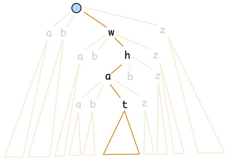
Imagine a giant tree made of letters. You start at the top (the root) and walk down one letter at a
time: W → h → a → t. Everything hanging below the spot where you stop is
a possible way to finish the word. So to suggest endings for "What", you walk to the "What" spot and look
at everything underneath it. That letter-tree is called a trie (say "try").
The classic data-structures answer to "find everything with this prefix" is a trie (a prefix tree). Each path from the root spells out a string, and shared prefixes share the same path — so "what is 2+2" and "what does the fox say" share the "what" branch.
What each trie node stores
- children — links to all the subsequent letters.
- isTerminal — does a complete search query end at this node?
- count — only meaningful when
isTerminal: the number of times this exact query has been searched.
class TrieNode {
    TrieNode children[63]     // a-z + A-Z + 0-9 + space
    long count;               // how many times has this
                              // query been searched
}
Why 63 children? Lowercase letters (26) + uppercase (26) + digits (10) + the space character (1) = 63 possible "next characters" at any node.
The read: typeahead(partialQuery)
To serve typeahead(partialQuery): start from the root and, for each letter of the
partial query, descend into the appropriate child. Once you reach the node that matches the
partialQuery, all possible suggestions live inside the subtree of that
node. To find the answer you'd have to walk that entire subtree (every query that matches the
prefix) and pick out the top 5.
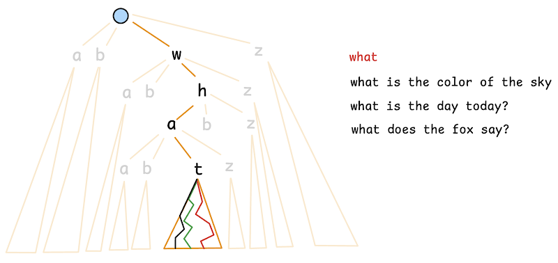
Walking the whole subtree is highly time-consuming. There are potentially billions of entries under a short prefix like "wh". Re-scanning that on every keystroke is a non-starter.
The fix: data-augmentation
We can fix this with data-augmentation: at every node, pre-compute and
store the top 5 results for that prefix. Now typeahead just reads the
already-computed answer off the node — no subtree scan at all. The price is that updates become
(slightly) slow, because writing a new count may change the stored top-5 of many ancestor nodes.
The node for "what" stores, right on itself:
["what is 2+2" → 10000, "what is the color of the sky" → 5000, "what does the fox say" → 2000].
When the user types "what", we walk four letters, land on the node, and hand back its stored list. No
billion-entry scan — just a four-step walk and a read.
The write: log_search(searchQuery)
To update the count for a query:
- Traverse to the node that matches this
searchQuery. - Increment its
count. - If augmented, also update the stored top-5 data for all nodes from here up to the root (because a bigger count here might now belong in the top-5 of every prefix above it).
typeahead(prefix) by walking the prefix and then
scanning the subtree for the top 5 — but that subtree can hold billions of entries. So we
data-augment every node with its pre-computed top 5: reads become instant, while writes
get a little slower because each new count must propagate up to the root.
3 Sharding a trie
One giant tree won't fit on one computer, so we cut it into pieces and put each piece on a different machine. The question is: how do we decide which piece a query belongs to? The rule we choose is the sharding key. We want each machine to hold a fair, roughly-equal share of the data — not one machine groaning under all the popular stuff while another sits nearly empty.
Q: What will be the sharding key? A sharding key decides which server (shard) a piece of data lives on. For a trie the natural choices are "first letter" or "first few letters" of the query.
Option A — shard by the first letter
Every query that starts with the letter a goes to the same shard. Important: this
does not mean the letter a gets a dedicated shard — a single shard
might contain several starting letters. We're only guaranteeing that all queries starting with
a land together in one place.
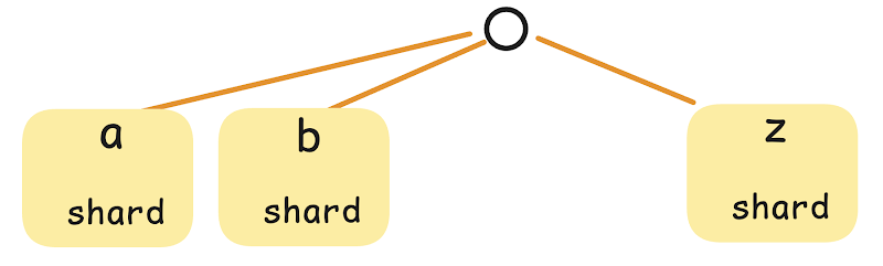
- Low cardinality — only 26 possible children, so at most ~26 groups to spread across machines.
- Uneven data distribution — the number of queries starting with
ais much higher than those starting withz. Some shards get swamped, others idle.
Option B — shard by the first 3 letters
Every query that starts with the letters abc goes to the same shard. (Same caveat:
a single shard may hold several starting triples; we only guarantee that all abc
queries are together.)
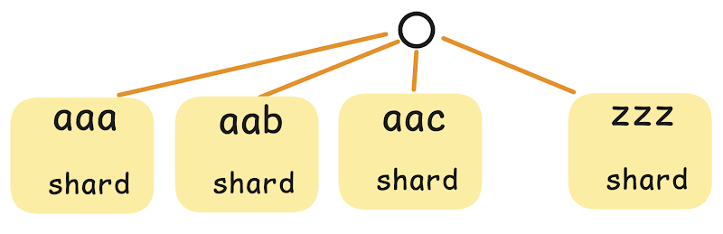
- High cardinality — 26³ ≈ 17,000 possible groups, so we have far more buckets to balance across machines.
- Still uneven — many more queries start with
whythan withzxz.
Fixing the load imbalance: manual grouping
To balance the load with the 3-letter key, we manually create groups of starting triples so that frequent prefixes get their own room and rare prefixes are clubbed together:
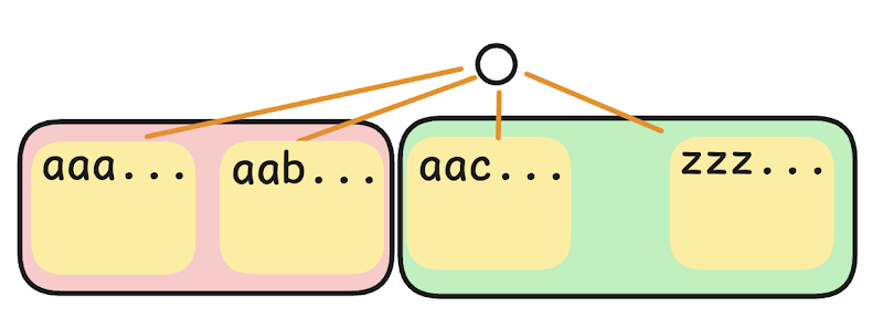
- Queries starting with
whyare very frequent ⇒ give them a dedicated shard. - Queries starting with
zxzare rare ⇒ group them with other rare prefixes (zyx+zxy+zxz+ …) onto one shard.
| Sharding key | Cardinality | Problem |
|---|---|---|
First letter (a → same shard) | Low — only 26 children | Very uneven: way more queries start with a than z. |
First 3 letters (abc → same shard) | High — 26³ ≈ 17,000 | Still uneven (why ≫ zxz); fix by manually grouping rare triples. |
There's no popular database built for storing tries. Tries exist only as a 3rd-party extension in some databases, but none was built specifically for them. So with this approach you'd have to build your own DB — which is exactly the pain that pushes us toward Approach 2.
4 Approach 2 — Hashmap / Key-Value
Forget the fancy tree. What if we just kept a giant cheat-sheet? On the left, every possible thing someone
might have typed so far ("wha", "what",
"what d"). On the right, the best few suggestions for that. When you type, we just
look up your row and read the answer — basically instant. That cheat-sheet is a
hashmap (key → value).
As a DSA person, we'd build a trie and augment each node with its top-5. As an HLD person
we realise we're effectively just caching the top-5 results for every possible prefix. So:
prefix == TrieNode and data-augmentation == cache. We can
drop the trie entirely and store this as a plain key-value cache!
Two databases
The design splits into two stores:
- Search Frequency DB — for each actual
searchQuery, store its count (how many times it's been searched). - Top Suggestions DB (cache) — for each possible prefix we'd show suggestions for, store the top-k suggestions.
Search Frequency DB (query → count)
| Search Query | Count |
|---|---|
| what is the color of the sky | 5000 |
| what is the day today | 1000 |
| what is 2 + 2 | 10000 |
| what does the fox say | 2000 |
| what does a fox eat? | 1900 |
| how to kill someone | 2000 |
| how to cook eggs | 1500 |
| how to sing | 500 |
Top Suggestions DB (prefix → top k = 3)
For each prefix we store the best 3 completions, already sorted by count:
wha
[
  what is 2+2                  => 10000
  what is the color of the sky =>  5000
  what does the fox say        =>  2000
]

what
[
  what is 2+2                  => 10000
  what is the color of the sky =>  5000
  what does the fox say        =>  2000
]
...

what i
[
  what is 2+2                  => 10000
  what is the color of the sky =>  5000
  what is the day today        =>  1000
]

what d
[
  what does the fox say        =>  2000
  what does a fox eat?         =>  1900
]

how
[
  how to kill someone          =>  2000
  how to cook eggs             =>  1500
  how to sing                  =>   500
]
...

how to k
[
  how to kill someone          =>  2000
]
The read: typeahead(partial_query)
If someone types "what i", we just go to the suggestions DB and look up that key.
This is very fast: hashmaps have O(1) lookup. (Technically it's
O(l) in the key length l — but keys in a hashmap should
never be long; if your hashmap keys are long, you're using hashmaps wrong.) Here the average key
length was assumed to be 10 chars and the max 50 chars. There's no
computation or processing needed — we just fetch the value for the given key.
Our non-functional needs: ultra-low latency (< 10 ms) and high read throughput (10 million reads/second at peak).
- A Redis lookup has latency
≤ 1 ms. ✅ - A single Redis server easily handles 100,000+ reads/writes per second.
- So we need only
~100 Redis serversto absorb 10M reads/s — trivial (Google had over 10 million servers as of 2020).
Sharding is now automatic — based on hash(key). And unlike tries,
there's a whole category of databases with first-class hashmap support. Q: Are there databases that
have first-class support for hashmaps? Yes — not just one, an entire category!
Key-value databases are basically hashmaps distributed across servers:
Redis / Memcached / DynamoDB / …
O(1) and Redis-fast (~100 servers for 10M reads/s).
Sharding is automatic via hash(key), and many real databases (Redis, Memcached,
DynamoDB) support this out of the box.
5 Logging searches & the write explosion
Every time someone finishes a search, we have to bump that query's popularity by one — easy. But because we pre-stored answers for every prefix, bumping one query also means re-checking the cheat-sheet rows for every prefix of that query: "wha", "what", "what d", and so on. One search turns into a whole stack of little updates. Multiply by a million searches a second and you get a problem.
Step 1 — update the count
Whenever someone searches "what does the fox say", we update the count in the
Search Frequency DB. Super simple: redis.inc(searchQuery).
Step 2 — update the cache (top suggestions DB)
Which entries need updating? If I'm updating the count for "what does the fox say",
could the suggestions for the prefix "how" change? No. Only the
prefixes of the search query itself are affected:
wha
what
what d
...
what does the fox
what does the fox s
what does the fox sa
what does the fox say
Suppose "what does a fox eat?" climbs from 1900 to 2100. It now
outranks "what does the fox say" (2000), so the affected prefixes are re-sorted:
what d
[
  what does a fox eat?         =>  2100
  what does the fox say        =>  2000
]

what do
[
  what does a fox eat?         =>  2100
  what does the fox say        =>  2000
]
The "wha" and "what" lists also pick up the new
higher-ranked entry.
The killer math: how many writes?
The average query is ~10 letters, so on average ~10 prefixes need updating per
log_search. That means each update is 1 + 10 = 11 writes
(1 to the frequency DB + 10 to the suggestions DB). Now scale it:
total redis writes
  = (1 million log_search / sec) * 11 writes / log_search
  = 11 million writes / second
We already needed 10 million reads/second for typeahead. Now we also need 11 million writes/second for logging. No database in the world is optimized for both heavy reads AND heavy writes at once. This tension is the central scaling problem — and we fix it in the next two topics.
log_search does one cheap count bump (redis.inc) plus an
update to every prefix of the query (~10 of them), so each search is ~11 writes. At 1M
searches/s that's 11M writes/s on top of 10M reads/s — making the system both read- and
write-heavy, which no single database handles well.
6 Optimizing reads & writes
A library that lots of people read from is easy — keep copies everywhere. A library where lots of people are constantly scribbling new notes is harder. A library where people both read tons AND scribble tons at the same time is a nightmare. The trick is to figure out which kind you have, and lean on a fast scratchpad (a cache) for the easy direction so the slow, careful book (the database) only does what it must.
Let's generalise beyond typeahead. How you optimize depends on whether the system is read-heavy, write-heavy, or both — and on whether you can tolerate eventual consistency.
If the system is read-heavy (not write-heavy)
- If eventual consistency is OK ⇒ absorb the reads in the cache, and optimize the DB for writes.
- If immediate consistency is needed ⇒ either:
- incur extra write latency with a write-through cache (your DB stays optimized for writes), or
- optimize the DB for reads — writes get slower (fine, there are few of them), and both reads & writes go to the DB. This is slower than the cached approach.
If the system is write-heavy (not read-heavy)
- Regardless of eventual vs immediate consistency ⇒ optimize the DB for writes.
- If your reads are significant, absorb them in the cache; if not significant, let them hit the DB and be slow.
- Your cache cannot handle the writes — a write-back cache would lose data if the cache server crashes with unsynced changes.
If the system is both read AND write heavy
This is very VERY difficult — and it's exactly our typeahead situation. Two escape routes:
- Reduce the writes:
- Batching — forces eventual consistency: wait for a bunch of requests to collect, then process them all in one go.
- Sampling — forces data loss: don't process all the requests, process only some of them.
- If you can't reduce writes, shard more. Sharding improves both reads & writes — but then you can't join across shards efficiently, so any query needing data from multiple shards is slow.
For typeahead we can afford eventual consistency and even some data loss — these are part of our non-functional requirements (suggestions only need to be relevant, not perfectly ranked or perfectly up-to-date). That permission is exactly what unlocks batching and sampling to crush the write load.
7 Reducing writes — batching & sampling
If 10 guests want tea, you don't boil one tiny cup, run it over, come back, boil the next — you make one big pot and serve everyone at once. That's batching. And if you want to know how a whole country voted, you don't ask all 1 crore people — you ask a small random handful outside polling booths and trust the trend. That's sampling. Both let us do far less work while still getting an answer that's good enough.
Because typeahead tolerates eventual consistency and data loss, we can use both tricks to shrink the 11 million writes/second down to something tiny.
Batching / batch processing
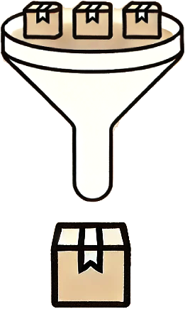
Instead of doing each task one by one, you wait for a lot of tasks to pile up, then do all of them in one go as a batch. (Example: 10 guests need tea — make individual cups one-by-one, or brew a whole pot at once and serve together. The pot is batching.)
For typeahead: whenever we get a log_search(search_query) request, instead of
updating the suggestions DB immediately, we wait for the count to increase by a fixed amount (say
1000) before pushing the suggestions update.
Earlier (no batching)
fn log_search(search_query):         // 1 million qps
    frequency_db.inc(search_query)      // 1 million writes/s
    update_prefixes(search_query)

fn update_prefixes(search_query):
    for i = 3 ... len(search_query) - 1  // 10 iterations
        prefix = search_query[:i]
        ... logic to update the suggestions list
            in the suggestions db
        // 10 million writes/s
With batching
fn log_search(search_query):         // 1 million qps
    updated_count = frequency_db.inc(search_query)
    // 1 million writes/s

    if updated_count % 1000 == 0:
        // update the prefixes only if the count
        // has changed by the batch size
        update_prefixes(search_query)

fn update_prefixes(search_query):
    ...   // (1 million / 1000 qps) * 10 updates
          // 10,000 writes/sec
Effectively, we only update the suggestions when the count increases by 1000.
Earlier: 1M writes/s (freq DB) + 10M writes/s (suggestions DB) = 11M writes/s.
After batching: 1M writes/s (freq DB) + (10M / 1000) = 1.01M writes/s.
We can't go below 1M/s — that's how often we must at least update the counts in the frequency DB.
Batching does not cause data loss — the frequency data is always up-to-date. It only causes delays (stale reads) in the suggestions updates.
Sampling
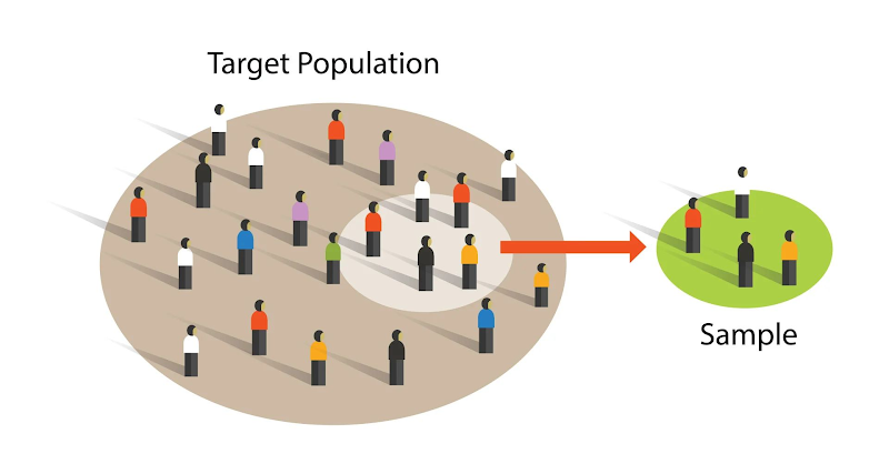
- A country-wide election has 1 crore voters; the actual counting takes several days.
- News channels want to predict the winner with high accuracy before the real results are announced.
- They can't talk to all 1 crore voters. Instead they stand in front of a small fraction of polling booths and, as people exit, ask a few random people "who did you vote for?".
- Using just that small subset/sample they estimate the winner. If the channel is unbiased, the exit-poll result almost perfectly matches the actual election result.
If you draw an unbiased sample from a population, then any trends that hold within the population will also hold within the sample. Typically a good way to get unbiased samples is to just sample uniformly at random.
Here's the architecture before and after. The search service is what calls the typeahead service's
log_search endpoint.
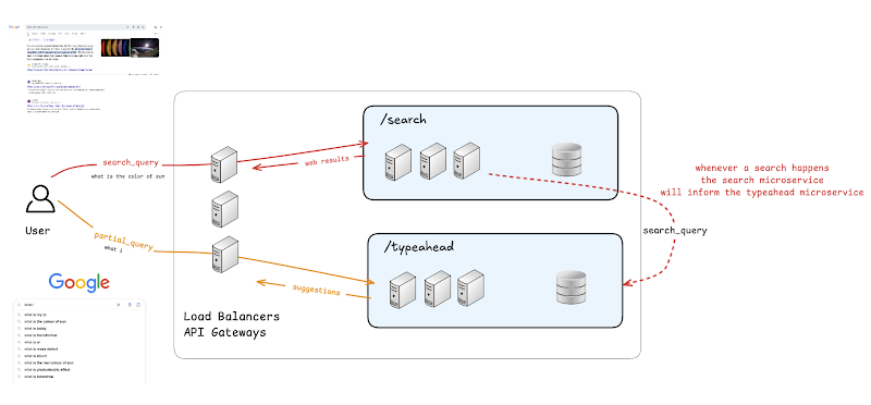
log_search on every search, so the typeahead service updates counts and suggestions for all of them.Earlier (every search logged)
// search service
fn search(query):
    ...
    make an API call to typeahead service's log_search endpoint

// typeahead service
fn log_search(search_query):
    frequency_db.inc(search_query)
    update_prefixes(search_query)

fn update_prefixes(search_query):
    for i = 3 ... len(search_query) - 1
        prefix = search_query[:i]
        ... logic to update the suggestions list
            in the suggestions db
With sampling
// search service
fn search(query):
    ...
    if rand() < 0.001:
        // with a probability of 0.1% make the following call
        make an API call to typeahead service's log_search endpoint

// typeahead service
    ...
For 99.9% of the searches, we don't even update the counts (we just ignore them). For a random
0.1% of searches, we call log_search and update both the counts and
the suggestions. Thanks to sampling, instead of 1M + 10M writes/second, we're back to
just (1M + 10M) / 1000 = 10,000 writes/second.
Won't the counts be inaccurate under sampling?
Yes — each count is effectively divided by approximately 1000 (not exactly, since it's random). But it doesn't matter: the suggestions shown to users stay highly relevant.
Won't the suggestions be slightly out of order?
Yes. And again it doesn't matter — relevance is preserved, which is all the feature needs.
With sampling, won't infrequent queries get tiny counts or be missed entirely?
Yes, that can happen — and it's a feature, not a bug! A rare query would never be part of typeahead suggestions anyway (because it isn't popular). Sampling automatically prunes the majority (99.9%) of the "bad" queries.
Sampling can lose individual data points, but it won't lose the overall trends. Use it only when data loss is okay.
8 Future scope — recency, geo, personalization, typos
A good autocomplete doesn't just know what's popular forever — it knows what's hot this week (recency), what people near you care about (location), what you personally search, and it forgives your typos. These extras turn a decent suggestion box into a great one.
Recency factor
Problem statement: when a big event happens — COVID lockdown gets declared, election
results are out, a high-profile person gets arrested, Federer wins Wimbledon — the query becomes
trending. Even though "why is the sky blue?" might have a higher
overall count, a trending "what happened in Nepal?" (recent + popular) should rank
higher when someone types "wh".
Approach 1 — separate counts per window
For each query keep three counts: Total, Last Week, Last Day.
total:why is the sky blue?    => 5000
 week:why is the sky blue?    =>  200
  day:why is the sky blue?    =>   50
total:what happened in Nepal? =>  500
 week:what happened in Nepal? =>  300
  day:what happened in Nepal? =>  100
To find the top-k: find top-k from total, find top-k from weekly, find top-k from daily, then merge the results using a scoring function. Goal: give more weightage to the recent counts.
Better solution — decay the historical counts
Simply decay the historical counts after every fixed period of time. For example, after each day, decrease the total count for each query by 10% (multiply by 0.9) before adding the day's new count.
"who has control over nukes?" gets a steady 1000/day:
[1000, 1000, 1000, …] — the raw total would be 100,000, but with decay:
day 1: 1000
day 2: 90% of 1000 + 1000  => 1900
day 3: 90% of 1900 + 1000  => 2710
day 4: 90% of 2710 + 1000  => 3439
...
day 100: 1000 * (1 + 0.9 + 0.9^2 + 0.9^3 + ...)
       = 1000 * 1/(1 - 0.9)
       = 10,000
So a forever-steady query converges to a decayed score of 10,000 (not 100,000).
"who won the wimbledon" is silent, then bursts:
[0, 0, …, 5000, 5000, 5000] — raw total just 15,000.
day 97: 0
day 98: 5000
day 99: 5000 * 0.9 + 5000   =>  9,500
day 100: 9500 * 0.9 + 5000  => 13,550
Its decayed score (13,550) now beats the steady query's (10,000) — recency wins. If a count after decay reduces below a threshold (say 0), we can remove that entry.
Geolocation-based personalization
- Given the user's request, find out their location based on IP address.
- Build a separate database for each location ⇒ shard the DB by
country_id. Now an Indian user's request only goes to the Indian shard.
"global: what does the fox say" => 1000
"India:  what does the fox say" =>   10
"USA:    what does the fox say" =>   10
When an Indian user types "wha", we find the suggestions for the
"wha" prefix and for the "India:wha" prefix, merge
the results, and return the final set.
User-based personalization
- Do this purely on the client side: the browser stores the user's search/browsing history.
- The browser creates typeahead suggestions from the user's local data.
- The browser also initiates a backend request to get the global typeahead suggestions.
- The browser merges these two lists.
- Google actually pulls this from the backend too — because it maintains your search & browsing history in its backend DB.
Handling typos
- Whenever a search is made, apart from updating the count of
search_query, also update the count ofspell_corrected(search_query). - Whenever a user types something, find the suggestions for
partial_query, but also include the suggestions forspell_corrected(partial_query).
def spell_corrected(input: str) -> str:
    """Corrects the spellings of the words within
       the input string, and returns the corrected
       string.
       Note:
           - each word in the input is spell corrected
           - gracefully handles partial words
    """
You can simply have a dictionary and calculate the edit-distance between the user's words and the words in the dictionary. Peter Norvig's classic essay "How to Write a Spelling Corrector" is the canonical reference for this.
spell_corrected() via edit-distance against a dictionary).
★ Putting it all together
You just designed a real, planet-scale autocomplete. Here's the one-paragraph story that connects every topic:
Typeahead must, on every keystroke, return the top queries that strictly start with the typed
prefix. A trie can do this if we augment each node with its
pre-computed top-5 — but no database stores tries, and sharding it evenly is painful. So we realise the
augmentation is just a cache and store everything as key-value: a
Frequency DB (query → count) and a Top Suggestions cache (prefix → top-k),
served from ~100 Redis servers at < 1 ms. The trouble is that every
log_search touches ~11 keys, making the system both read- and write-heavy
(10M reads/s + 11M writes/s) — which no DB handles. Because typeahead tolerates eventual consistency and data
loss, we crush the writes with batching (update only every 1000th count → ~1.01M writes/s,
stale but lossless) and sampling (log a random 0.1% → ~10k writes/s, lossy but
trend-preserving). Finally we make it smart with recency decay, geo-sharding,
client-side personalization, and typo correction via edit-distance.
Quick self-check
Why is scanning a trie subtree on every keystroke a bad idea, and what fixes it?
A short prefix can have billions of entries in its subtree, so scanning it per keystroke is far too slow. The fix is data-augmentation: pre-compute and store the top-5 at every node, so a read just reads the node. The cost is that writes must propagate the new count up to the root.
Why move from a trie to a key-value store?
Augmenting a trie is really just caching top-k per prefix, so prefix ==
TrieNode and augmentation == cache. Unlike tries (no off-the-shelf DB
supports them, sharding is uneven), key-value stores like Redis/Memcached/DynamoDB give O(1) lookups,
automatic hash(key) sharding, and first-class support.
Why does log_search create such a heavy write load?
Each search bumps the count (1 write) and must update the cached top-k for every prefix of the query (~10 writes), so ~11 writes per search. At 1M searches/s that's ~11M writes/s — combined with 10M reads/s, the system is both read- and write-heavy, which no single DB optimizes for.
Batching vs sampling — what does each cost you?
Batching only updates suggestions every Nth count (e.g. 1000), giving ~1.01M writes/s; it causes stale reads but no data loss (counts stay exact). Sampling logs only a random 0.1% of searches, giving ~10k writes/s; it causes data loss of individual points but preserves overall trends (and usefully discards rare queries).
How do we make a trending query outrank a stale all-time-popular one?
Apply recency decay: each day multiply existing counts by 0.9 before adding the new day's count. A steady 1000/day query converges to 10,000, while a fresh burst (e.g. Wimbledon) can shoot past it (13,550) — so recent popularity wins. Entries that decay below a threshold are removed.
📚 References & Further Reading
Class material
- 📄 Original class notes / handout (Google Doc) — open the shared class material for this session.
- Class handout: "[SST-2028] Case Study: Typeahead -2".
Papers, docs & deep dives
- 📄 Peter Norvig — How to Write a Spelling Corrector — the edit-distance approach behind typeahead typo handling.
- 📄 Redis documentation — the in-memory key-value store powering the suggestions cache (< 1 ms lookups, 100k+ ops/s per server).
- 📄 Amazon DynamoDB — a managed distributed key-value database, automatic
hash(key)sharding. - 📄 The System Design Primer — broad reference on caching, sharding, and read/write-heavy optimization patterns.